
CBM of Compressors Using Tobu Railway’s Remote Online Monitoring SystemImproved Filtering to Shorten Time Taken to Acquire Enough Data for Detection
Highlight
Advances in ICT have enabled the railway industry in recent years to introduce the online monitoring of trains, with data such as onboard operation records being transmitted wirelessly in real time. This has led Hitachi to pursue the study and collaborative creation of technologies that use this data for the condition-based maintenance of onboard equipment.
As one example of this work, this article describes a technique for detecting potential faults in compressors, including the process by which the data required for anomaly identification is obtained and what has been done to shorten the time required.
1. Introduction
Recent advances in information and communication technology (ICT) have enabled the online monitoring of trains, with data such as onboard operation records being transmitted back to the control center wirelessly in real time. A typical example of this is the transmission of data from the train control and monitoring system (TCMS) on the E235 commuter trains of the East Japan Railway Company (JR East) using Worldwide Interoperability for Microwave Access (WiMAX) communications1). As this data contains a wide range of information on train operation and the state of the rolling stock, extending its use beyond events like accidents or equipment failures has the potential to add value to railway systems in other ways such as lower maintenance costs.
Remote is a WiMAX-based online monitoring system that was developed by Tobu Railway Company, Ltd. and Hitachi. It was first deployed in 2019 on three WiMAX-equipped 60000 Series trains operated by Tobu Railway. The system was also installed on six of Tobu Railway’s 60000 Series trains and five 50000 Series trains in 2023, this time using the Long-Term Evolution (LTE) communication standard. One of the ways in which the onboard data acquired by Remote is being put to use is that the companies are working on the collaborative creation of condition-based maintenance (CBM) techniques for rolling stock systems. This article describes a technique for detecting potential faults in compressors that forms part of this work, including the results of work done to shorten the time taken to acquire the data needed to identify anomalies so that methods developed using data from the WiMAX rolling stock can be deployed on the LTE rolling stock, for which there is little data available yet.
2. Overview of Remote
Figure 1—Block Diagram of Remote System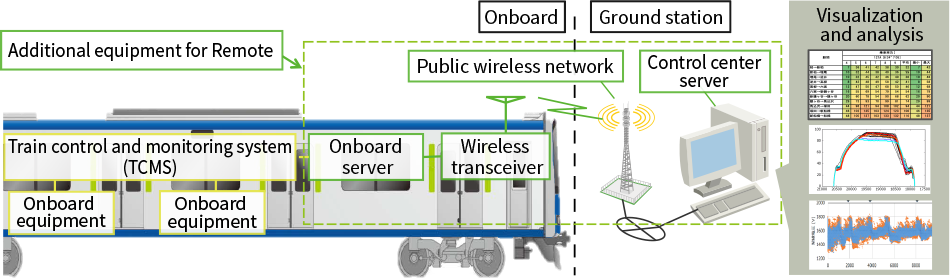 TCMS: train control and monitoring systemThe Remote system is made up of an onboard server, wireless transceiver, and control center server. The train’s TCMS connects to the onboard server to send rolling stock data to the control center server.
Figure 1 shows a diagram of the Remote online monitoring system adopted by Tobu Railway. Trains have a TCMS for passing information between different equipment. The Remote system augments this with an onboard server and wireless transceiver, transmitting data to a control center server via a public wireless network. The transmitted information includes train location, speed, driving data, and air suspension (AS) and brake cylinder (BC) pressures. This article explains how this information is used to identify signs of potential faults in railway compressors.
3. Overview of Railway Compressors and Potential Faults
Compressors are used in trains to provide compressed air for operating the onboard pneumatic systems (such as air brakes and air springs). While both oil-filled and oil-free compressors are used in the industry, this study focused on the oil-filled compressors fitted in Tobu Railway’s 60000 Series and 50000 Series rolling stock that use the Remote system.
Figure 2—Block Diagram of Pneumatic System and Definition of Operating Time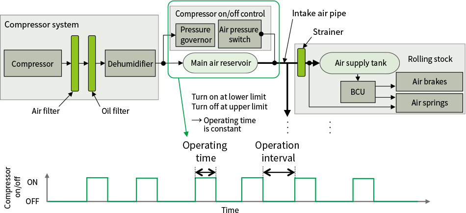 BCU: brake control unitThe pneumatic system is made up of a compressor and the equipment that uses the compressed air it generates, such as air brakes and air springs. For the analyses described in this article, the operating time is defined as the time from the compressor starting up until it shuts down and the operation interval is the time until it next starts up again.
Figure 2 shows a diagram of a pneumatic system that incorporates a compressor. The compressor starts up whenever the tank pressure of the air reservoir falls below the lower limit and shuts down once the pressure reaches the upper limit. Accordingly, provided there are no external factors involved, the compressor should always run for the same length of time. If, on the other hand, there is a fault such as an oil leak or low oil level, the operating time will be longer due to the loss of air compression performance or ability to build pressure. In other words, the detection of longer operating times can warn of a potential fault. However, there are also situations in which a compressor that is working normally will still have a longer operating time, for instance when compressed air is used by pneumatic equipment such as brakes or air springs while the compressor is running. This means that the increase in air demand from such equipment needs to be taken into account if potential faults are to be detected based on increases in operating time.
4. How to Detect Potential Compressor Faults and Associated Challenges
4.1 Overview of Previous Method
It is assumed that the amount of air used by brakes and air springs can be estimated based on the changes in equipment pressures and other information such as railway line topography. On this basis, the compressor is deemed to be operating abnormally if the difference between the actual and estimated operating times is large, with the estimated time being the mean value determined from the air consumption conditions. These are the BC and AS pressure variations (the cumulative changes in the BC and AS pressures during compressor operation) and four conditions for the location of the train when the compressor starts and stops operation that serve as an indicator of the topography. Data from the WiMAX-equipped rolling stock had already been used to develop a method for identifying potential compressor faults in this way2). Figure 3 shows how this works.
Figure 3—Method for Detecting Potential Compressor Faults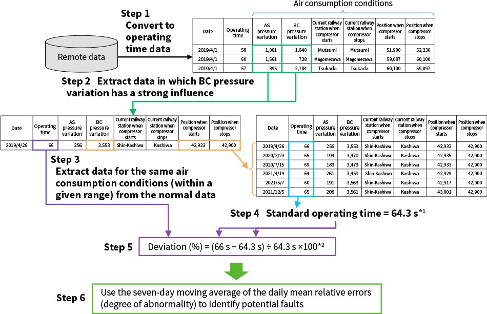 AS: air suspension, BC: brake cylinder
*1 The mean value for normal operation is used as a standard benchmark.
*2 As it is known that operating times tend to be longer when the compressor has a problem, the method substitutes a value of zero when the relative error is negative.The method uses a five-step process (steps 1 to 5) to identify potential faults.
- Step 1:
- Convert and collect Remote data as operating time data (operating times and calculated air consumption conditions*1)).
- Step 2:
- From the collected data, extract data strongly influenced by BC pressure variation that are closely correlated with operating time (BC pressure variation ≥ 2,000 kPa and AS pressure variation ≤ 300 kPa).
- Step 3:
- For operating time data TX, from the data obtained in Step 2, identify data for which the air consumption conditions (BC pressure variation and train location) are within a given range*2).
- Step 4:
- If five or more data points are identified in Step 3*4), calculate the mean operating time and use this as the standard operating time (TSt).
- Step 5:
- Use equation (1) to calculate the TX deviations relative to TSt.
Equation (1) Deviation (%) = (TX − TSt) ÷ TSt × 100 - Step 6:
- For days on which there were five or more data, and deviations were calculated in Step 5*3), calculate the mean deviations for each day (degree of abnormality) and use this to determine whether an abnormality is indicated. To prevent misdetection due to outlier values, this study used a moving average of the degree of abnormality with a time period long enough to cope with the variability of daily operation (typically seven days).
- *1)
- The AS and BC pressure variations used as air consumption conditions are defined as follows. Here, ts is the compressor start time, tf is the compressor stop time,
is the five-second moving average of the pressure, and
is the one-second moving average of the pressure.
Equation (2)
Equation (3)
- *2)
- The BC pressure variation is less than or equal to the variation in value likely to occur due to sensor error and the difference in the compressor start time and stop time positions is less than or equal to the length of the train.
- *3)
- The thresholds for the number of data points in Steps 4 and 6 were the values that achieved the best detection in past studies.
4.2 Issues with Previous Method
The method described above includes filtering in Step 2 to exclude some data from detection. This means that a large quantity of data must first be collected to ensure that there will be enough to satisfy the thresholds in Steps 4 and 6. This posed a problem when migrating the technique to new rolling stock such as LTE-equipped trains, for which data only started being collected in FY2023. Figure 4 shows the results for one of these LTE-equipped trains, the 61610 trainset (for which approximately nine and a half months of data had been collected as of May 2024). Specifically, the figure shows the performance of the previous method when the data collection period was varied in two-month increments, the number of data points for each of these periods, and whether or not they were sufficient for the method to be used. These results indicate that, whereas the eight-month data closely tracks the data collected over nine and a half months and so should be adequate for detection, the data collected over six months or less cannot be used because it includes periods where they diverge. The trains with the shortest data collection period as of May 2024 were the 50000 series LTE rolling stock, for which there was only about six months of data. Accordingly, the requirement for the preliminary data collection period needed to be shortened to less than six months if the newly developed technique for detecting potential faults was to be used on all LTE trains.
Figure 4—Example Application to Long-Term Evolution (LTE) Rolling Stock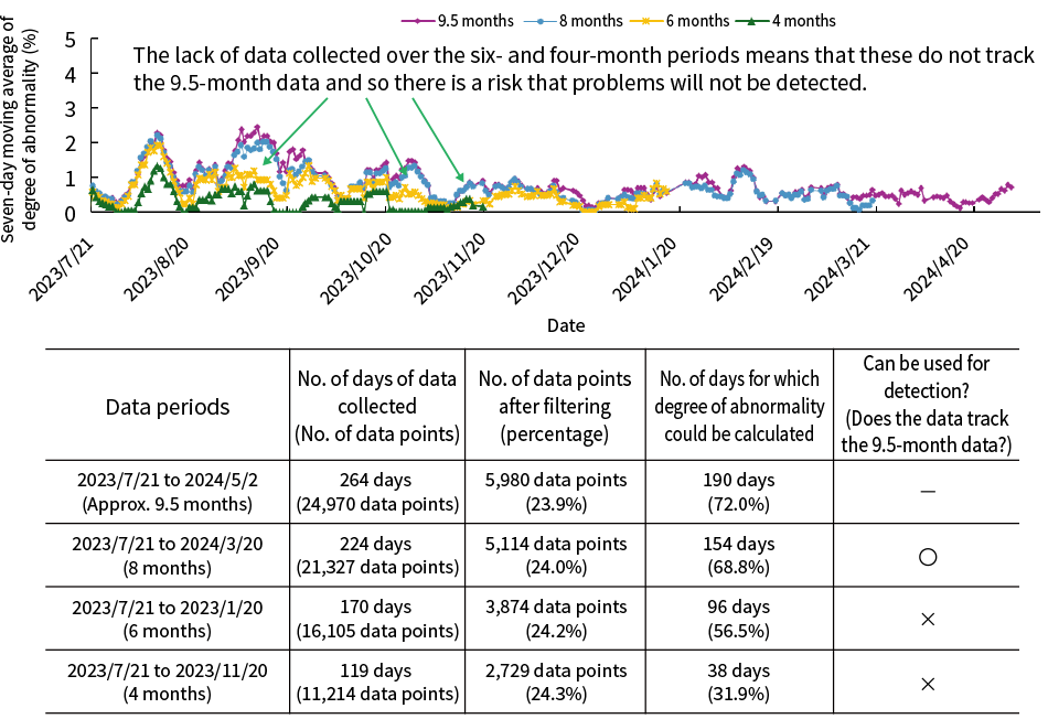 When used on LTE-equipped rolling stock, the previous method required eight months of data collection before it could detect potential faults.
Next, whereas the eight-month data listed in Figure 4 consisted of about 5,000 data points after filtering, and given the degree of abnormality that could be calculated for 68.8% of the days, the six-month data consisted of about 4,000 data points after filtering and the degree of abnormality could be calculated for 56.5% of the days. That is, when the quantity of collected data is small, the number of usable data points after filtering will likewise be small and the number of collected data points selected in Step 3 will be lower. This will increase the number of data points for which a standard time cannot be calculated in Step 4 and reduce the number of days for which a degree of abnormality can be calculated, meaning that there will be an increasing number of occasions when two or more days are missing from the seven-day moving average calculation. As a value of zero is used for the degree of abnormality on these missing days, the degree of abnormality will be under-estimated because multiple days are missing. This is one of the reasons why the trend in the degree of abnormality is out of step for data collection periods of less than six months, as occurs in Figure 4. What is needed, then, is to improve filtering so that fewer collected data points will be needed for detection to work. That is, improved filtering will enable a higher proportion of the collected data points to be used.
5. Improved Filtering
5.1 Filtering Used in Previous Method and How to Reduce Filtering Data Loss
This section describes how filtering was performed previously. It was found that the AS and BC pressure variations used as air consumption conditions correlate weakly and strongly, respectively, with operating time. Accordingly, to improve the accuracy of the standard operating time calculation in Step 4, data was identified for which the compressor is operating and air consumption is high for the brakes, but low for the air springs. This provides data with a strong correlation between air consumption conditions and operating time. In the case of the 60000 Series, the mean value for the BC pressure when a single brake is engaged is about 160 kPa. As each train has 12 BC pressures, the brakes are assumed to be engaged if the pressure exceeds about 1,920 kPa (160 × 12). On this basis, a threshold of 2,000 kPa or higher was defined for the BC pressure variation. Meanwhile, an analysis of high values of AS pressure variation found instances where air pressure was consumed to maintain the rolling stock height when the weight on the springs changed due to large changes in passenger load, something that occurs when the train is stopped, which was found to influence the operating time. Accordingly, the analysis identified the range in which AS pressure variations have little influence on operating time (when the correlation between AS pressure variation and operating time is weakest) and used this to define a threshold of 300 kPa or less for the AS pressure variation. As a result, increasing the number of data points available after filtering requires finding ways to use data where the AS pressure variation is over 300 kPa and the BC pressure variation is under 2,000 kPa.
To allow more data through filtering, an analysis was performed to identify circumstances under which AS pressure variations have a weak correlation with operating time. Each bogie has two air springs and a differential pressure valve or similar is used to distribute air between them when the train is moving. On the 60000 Series, however, information on AS pressure is only acquired from one of these. This means that, when the AS pressure variation increases, it is impossible to distinguish between cases where air was consumed and therefore the operating time increased and cases when air was redistributed between the two springs, as above, and the operating time did not increase. This is one of the reasons for the weak correlation between AS pressure variation and operating time. However, if only times when the train is stationary are considered, the air springs consume air in response to changes in the number of passengers, as explained above about data for ranges when the AS pressure variation is large. As this involves a change in air pressure across all air springs in a car simultaneously, it does affect the operating time. From this it was concluded that the likelihood of a correlation between AS pressure variation and operating time will be high if only the data from stationary trains is used.
Figure 5—Relationship between AS Pressure Variation and Operating Time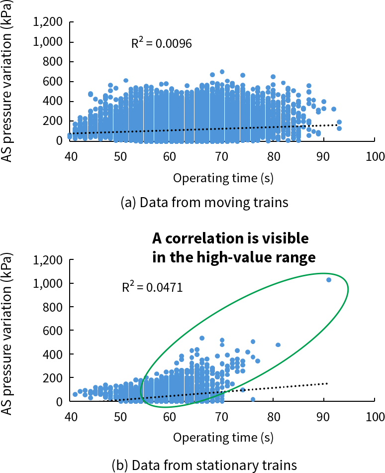 No correlation between the operating time and AS pressure variation is visible in data where the compressor is operating in a moving train but a correlation is visible in data where the compressor is operating in a stationary train.
To confirm this hypothesis, approximately three years of data from the WiMAX-equipped 61616 trainset used to develop the technique (64,842 data points) was separated into two datasets where the compressor was operating in a moving or stationary train, respectively. The correlation with operating time was then determined for each dataset. The results are shown in Figure 5. The best-fit lines shown in the graphs were obtained by least-squares linear approximation. The coefficient of determination for the moving-train data shown in graph (a) was 0.0096, equivalent to a correlation coefficient of 0.098. This indicates almost no correlation between AS pressure variation and operating time. For the stationary-train data shown in graph (b), on the other hand, the coefficient of determination of 0.047 gives a correlation coefficient of 0.22, indicating a weak correlation between AS pressure variation and operating time. In particular, data that appears to show a correlation with operating time is visible in the range where the AS pressure variation values are high. From this it was concluded that the number of usable data points could be increased by treating data from moving and stationary trains differently in terms of their filtering and air consumption conditions. The following section presents the results of a study into a method that separates the data from moving and stationary trains in the previous method’s Step 2 (filtering data to use in subsequent steps) and Step 3 (using air consumption conditions to extract past data).
5.2 Study of Filtering and Air Consumption Conditions for Data from Moving Trains
The study looked at filtering and air consumption conditions for moving-train data. Analysis found a strong correlation between BC pressure variation and operating time, with a correlation coefficient of 0.81. On the other hand, there was almost no correlation between AS pressure variation and operating time in moving-train data, as shown above in Figure 5(a). In this regard, the relationships in moving-train data between BC pressure variation and operating time and between AS pressure variation and operating time are the same as the previous method. This is because moving-train data makes up about nine-tenths of all operation data. While data strongly influenced by BC pressure variations is still used in the case of moving-train data, as was the case for the previous method, the aim is to increase the quantity of data by relaxing the filtering based on BC pressure variation. Also, as it is assumed that the effect of AS pressure variation on operating time is only small for data from moving trains, there is no filtering based on AS pressure variation.
Next, the trend in BC pressure during braking was assessed to investigate BC pressure variation filtering. The analysis found the change in BC pressure to be about 100 kPa at the start of deceleration. That is, when each BC pressure is 100 kPa or more, it indicates that the consumption of air for braking has started. From this it was concluded that a value of 100 kPa multiplied by the number of BC pressure measurements was appropriate for filtering based on BC pressure variation. As 12 BC pressure measurements (two measurements per car × six cars) are acquired for the 60000 Series rolling stock of Tobu Railway that were the subject of this study, a value of 1,200 kPa (100 kPa × 12) was adopted for filtering.
Next the air consumption conditions were considered. As moving-train data accounts for about nine-tenths of all operating data, as noted above, the correlations between the BC and AS pressure variations and operating time remained the same as for the previous method. Accordingly, the air consumption conditions were treated the same way as in the previous method, with the BC pressure variation and train location being used.
5.3 Study of Filtering and Air Consumption Conditions for Data from Stationary Trains
A new study was conducted into filtering and air consumption conditions for stationary-train data. This began with a review of AS pressure variation filtering. As shown in Figure 5(b) above, AS pressure variations in stationary-train data show a correlation with operating time in the high-value range. Accordingly, data that has a strong correlation with operating time can be extracted by filtering based on whether the values indicate that changes in AS pressure are associated with air consumption.
No AS pressures are acquired in the data from the 61616 trainset and other WiMAX rolling stock and they are instead back-calculated from the passenger load. On this basis, the threshold was set based on values for which the passenger load was assumed to have varied. As the base AS pressure data has a resolution of 5 kPa/bit, a variation of ±5 kPa is always present due to sensor error. When AS pressure is converted to passenger load, 5 kPa corresponds to about 1%. Also, the passenger load data was found to have a background fluctuation of ±1%. Accordingly, a change in passenger load is deemed to have occurred when there is a variation of ±2% or more. As the passenger load data has a resolution of 1%/bit, the conversion of AS pressure to passenger load is rounded to the nearest whole number. As a result, when passenger load is converted to AS pressure, the conversion error is such that 1% of passenger load corresponds to 4 to 6 kPa. Converting a ±2% variation in passenger load to AS pressure on this basis gives a change of ±12 kPa or more. A single value for passenger load is obtained from each car, meaning that six data points are obtained for the six cars in 60000 Series trains. From this, a value of 12 kPa × 6 (72 kPa) is deemed to indicate a change in all AS pressures. In the case of LTE rolling stock, however, actual AS pressures are acquired and so these measured values are used instead. As sensor error for the AS pressures in LTE rolling stock is ±5 kPa, a variation of 10 kPa in a single AS pressure data point is deemed to indicate a change. As each LTE car has two AS pressure measurements, a change is defined as a variation of more than 6 × 2 × 10 kPa (120 kPa). On this basis, a filter setting of 72 kPa was used for WiMAX rolling stock and 120 kPa for LTE rolling stock.
The next step was a review of BC pressure variation filtering. As indicated by equation (3), BC pressure variations are acquired from five seconds before the compressor starts up. Excluding those cases when the compressor starts up after the train has been stationary for a long time, changes in BC pressure also include cases due to braking immediately prior to the train stopping. On this basis, it was concluded that a filter threshold of 1,200 kPa would be appropriate, the same as for moving-train data.
The final step was a review of air consumption conditions. As noted above, air consumption caused by passengers getting on or off the train should be strongly correlated with operating time and therefore it is appropriate to use AS pressure variation as an air consumption condition. Moreover, unlike for moving-train data, train location is not applicable to stationary trains as they do not move. However, as the size of variations may exhibit characteristics that depend on the orientation of the train due to the topography of the station (whether the track is curved or sloped), station name is also used as an air consumption condition. Also, as BC pressure variation affects the operating time (being a cumulative value starting from five seconds before the compressor starts), it is also used as an air consumption condition.
5.4 Overview of New Method
The method considered in the above two sections deals with the data for moving and stationary trains separately. This section looks at how it differs from the previous method. Figure 6 provides an overview of the previous and new methods. The biggest difference between the two methods is that the new method uses different filtering and air consumption conditions for data from moving and stationary trains, respectively. For data from moving trains, the air consumption conditions are determined the same way as before. Instead, the number of data points has been increased by ignoring the AS pressure variations when filtering and by changing the filter setting for BC pressure variations. For stationary-train data, the new method differs from the previous method in that it uses AS pressure variation to determine whether air consumption occurs. This has enabled the number of data points to be increased by using data with high values of AS pressure variation, something that was not a consideration in the previous method. These changes have increased the amount of usable data by roughly half, from about 40% of all data points to about 60%. The following sections assess the calculation accuracy based on the error rates for the previous and new methods and confirm the benefits of increasing the number of data points.
Figure 6—Comparison of Previous and New Methods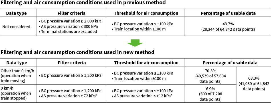 * For LTE rolling stock, the filter setting for AS pressure variation is 120 kPa or more and the threshold for identifying air consumption is a change in AS pressure of ±10 kPa or less.The new method uses different filtering to suit data from moving and stationary trains, respectively.
6. Assessment Using Actual Data of Shortening of Data Collection Period
6.1 Comparison with Detection Accuracy for WiMAX Rolling Stock Data
The following two comparisons with the previous method were performed to assess the extent to which the increase in the number of data points provided by the new method changed the accuracy of the degree of abnormality calculation and anomaly detection.
- Comparison of calculation accuracy for seven-day moving average of degree of abnormality
- Comparison of trends in seven-day moving average of degree of abnormality
These comparisons used the seven-day moving average of degree of abnormality, the same criterion that is used for detection. The accuracy was assessed using data from three WiMAX trains (the 61616, 61617, and 61618 trainsets).
- Comparison of calculation accuracy for seven-day moving average of degree of abnormality
The means and maximums of the seven-day moving average values obtained by the previous and new methods were compared using data from three WiMAX trains. The results are listed in Table 1. In all cases, the calculations were performed using datasets that excluded the month preceding oil replenishment and other maintenance work on the trains. Such datasets are referred to below as “normal data.” As shown in Table 1, the mean value for the new method increased by between 0.04 and 0.09% and the maximum by between 0.11 and 0.40%, indicating a small deterioration in calculation accuracy. However, as the mean operating time for the 60000 Series is about 65 seconds, 0.09% of the mean corresponds to 0.06 seconds and 0.40% of the maximum translates to a difference in operating time of only 0.26 seconds. As operating time is acquired in one-second increments, a 0.26-second difference in the maximum is less than the operating time detection accuracy. Based on this, it was concluded that the new method has similar calculation accuracy to the previous method. - Comparison of trends in seven-day moving average of degree of abnormality
Graphs (a) to (c) in Figure 7 compare the trends in the seven-day moving average values for degree of abnormality obtained by the previous and new methods using data from three WiMAX trains. Overall, the rises and falls in the degree of abnormality followed the same trend for all trainsets, with the threshold set for the previous method based on the maximum value during normal operation being exceeded at the same timings for both the previous and new methods, indicating successful detection of oil replenishment. These results indicate that the new method can provide similar detection accuracy to the previous method.
This assessment indicates that using the new method to relax filtering and provide more data points still achieves similar detection accuracy to the previous method.
Table 1—Comparison of Calculation Accuracy for Degree of Abnormality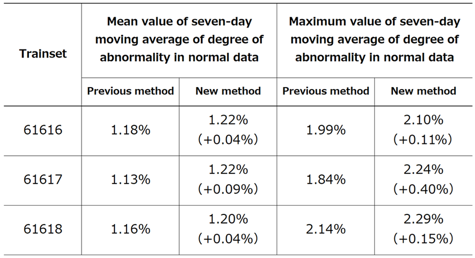 The comparison shows that the difference in the degree of abnormality calculation accuracy between the new and previous method is less than the operating time measurement error and that using the new method achieves similar detection accuracy to the previous method.
Figure 7—Comparison of Trends in Seven-day Moving Average of Degree of Abnormality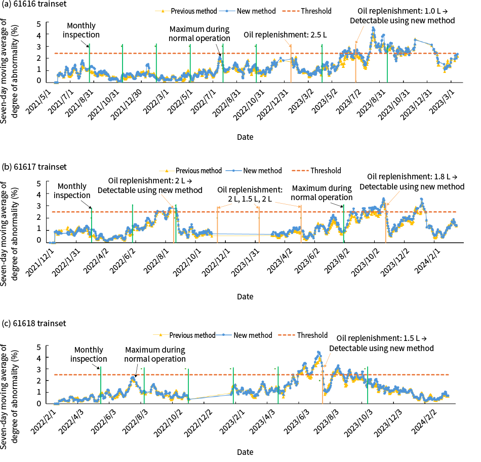 The trend in the degree of abnormality does not change between the previous and new methods.
6.2 Assessment of Benefits Based on LTE Rolling Stock Data
Figure 8—Relationship between Number of Pre-filtering Data Points and Percentage of Days on which Degree of Abnormality Can be Calculated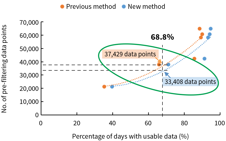 As the 61616 trainset generates about 80 data points a day on average, a reduction of about 50 days is anticipated, from 467 days (37,429/80) for the previous method to 417 days (33,408/80) for the new method.
Figure 9—Comparison of Previous and New Methods Applied to 61610 Trainset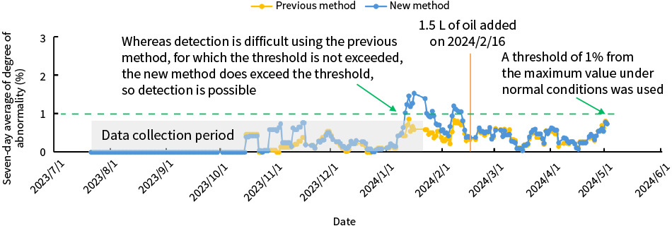 The results show how events that would be difficult to detect during the data acquisition period using the previous method can be detected using the new method.
An assessment was performed to determine the extent to which the increased number of data points provided by the new method can shorten the data collection period.
The results shown in Figure 4 indicate that, for 60000 Series LTE rolling stock, anomaly detection is possible if a degree of abnormality can be calculated on 68.8% of days. On this basis, an estimate was made of the number of days by which the data collection period could be shortened. Figure 8 shows a graph that plots the number of input (pre-filtering) data points against the percentage of days on which the degree of abnormality can be calculated for the previous and new methods, respectively. Using the best-fit lines in the graph, calculating the number of days for which the degree of abnormality can be obtained indicates that about 50 fewer days worth of data are required to achieve this 68.8% level of performance. If the required data acquisition period can be shortened by 50 days, a result can be obtained for LTE rolling stock in 174 days (about six months), down from the requirement of 224 days indicated in Figure 4.
Next, an assessment was performed to determine whether anomaly detection would work in practice for LTE rolling stock assuming a six-month data collection period. The LTE rolling stock includes data for the 61610 trainset for which maintenance records indicate that oil replenishment and other maintenance work was performed shortly after the data collection period. Figure 9 shows the results when the previous and new methods were applied to this data. Data acquisition from the 61616 trainset commenced on July 21, 2023 and continued until January 20, 2024, with a top-up of 1.5 L of oil occurring shortly after that on February 16. On this basis, the data obtained after oil replenishment was treated as representing normal conditions and a threshold of 1.0% from the maximum value was adopted. While the results for the previous method shown in Figure 9 indicate that detecting when oil replenishment occurred would be difficult as the threshold was not exceeded in the period prior to this happening, the results for the new method do exceed the threshold, so detection is possible.
These studies indicate that anomaly detection is possible using the new method with a data collection period of only about six months and that anomaly detection should be usable even on the 50000 Series LTE rolling stock, which have the shortest data collection period.
7. Conclusions
This article has described a review of the filtering used in a potential fault detection technique for the CBM of railway compressors that uses rolling stock data acquired by the Remote system, the goal being to shorten the data collection period needed for anomaly detection. The study demonstrated that filtering data from moving and stationary trains separately in ways that best suit each dataset can increase the amount of usable data by preventing data from being rejected unnecessarily, thereby shortening the preliminary data collection period by about 40 days. When applied to data from operating trains, it was found that potential fault detection could be performed on LTE rolling stock after a six-month data acquisition period, indicating that the technique could be used on the 50000 Series LTE rolling stock, which has the shortest data collection period.
In the future, Hitachi intends to deploy the technique on LTE-equipped and other new rolling stock and to undertake further work on the automatic generation of detection criteria as well as improvements to detection accuracy.
REFERENCES
- 1)
- N. Nakamura, et al., “Overview of JR East's Type E235 Next-Generation Commuter Train,” Journal of The Society of Instrument and Control Engineers, pp. 138 - 141 (Feb. 2017) in Japanese
- 2)
- S. Kitai, et al., “Study of compressor failure prediction detection technology using monitoring data of train,” Proceedings of the 2024 National Conference of the Institute of Electrical Engineers of Japan (4), pp. 279 - 280 (Mar. 2024) in Japanese